I had a colleague involved with the International Year of the Salmon (IYS) ask why this zooplankton dataset from the IYS expeditions was referenced in a paper that seemed to be about terrestrial species(garcía-roselló2023?). It’s not immediately obvious how the IYS zooplankton dataset was used in this paper, but if you dig in a little deeper it becomes clear, and frankly amazing, how GBIF integrates data and counts citations.
How was the IYS Zoop Data Used?
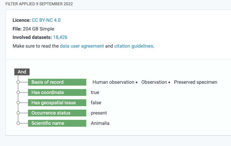
If you look in the references section of the Garcia-Rosello et al. (2023) paper you will see two links to GBIF Occurrence Downloads. If you click on the DOI for the second GBIF Occurrence Download dataset (GBIF.Org User 2022), you will reach a landing page for an Occurrence Download on GBIF from a specific query made by a user. You can even see the specific query filters that were used to generate the dataset.
The query filters generated by a GBIF user to return an integrated dataset
A total of 18,426 datasets that meet the query filter. The filter included: has CC BY-NC 4.0 licence, Basis of record must be either Human observation, Observation or Preserved Specimen, Has coordinate is true, … Scientific name includes Animalia). As it turns out, this is a very broad filter basically asking for all the animal occurrences on GBIF datasets that have the right license and metadata and the IYS dataset about zooplankton met all those criteria. If you wanted to see all the datasets included in the new dataset you can download a list of the involved datasets using the “Download as TSV” link from the GBIF Occurrence Dataset landing page for this big dataset and search for International Year of the Salmon to see which datasets are included.
So the dataset that resulted from this specific query includes data from 18,426 other GBIF datasets which meet the query filter parameters. This new dataset receives a Digital Object Identifier and each of those underlying datasets also has a digital object identifier. GBIF is able to count citations because each of those 18,426 DOIs is referenced in the new dataset’s DOI metadata as a ‘relatedIdentifier’. So, each time the overarching dataset is cited, the citation count for each of the 18,426 datasets increases by one as well. Pretty cool, huh!?
I can be surprising how the International Year of the Salmon data are re-used way outside the context of their collection, which is a major advantage of using the GBIF and publishing data using international standards. This also demonstrates the power of standardized data: new datasets can be integrated, downloaded, and identified with a DOI on the fly!
If you’re interested in finding all 18,427 Digital Object Identfiers and their titles or other metadata here’s how you could do that using the DataCite API and the rdatacite R package and searching for the DOI of the overarching dataset and extracting the relatedIdentifiers field.
International Year of the Salmon Datasets
For a more interesting example, let’s look at how all the International Year of the Salmon datasets have been cited thus far. To do that we’ll take a similar approach but instead of searching for a specific DOI we’ll query for International Year of the Salmon in all the datacite DOIs, and extract each datasets relatedIdentifiers. We’ll then search for those relatedIdentifiers to retrieve their titles. Finally, I’ll join all that data together and present a network map of how each dataset connected by citations.
Code
library(rdatacite)library(tidyverse)library(networkD3)# download the DOI metadata for the new overarching datasetgbif_doi <-dc_dois(ids ="10.15468/dl.cqpa99")datasets_used <- gbif_doi[["data"]][["attributes"]][["relatedIdentifiers"]][[1]]["relatedIdentifier"]# Get the data from 'International Year of the Salmon' titlesiys_dois <-dc_dois(query ="titles.title:International Year of the Salmon", limit =1000)# Create a tibble with the title, citation count, and DOI for each record, then filter by citation count greater than 0iys_citations <-tibble(title =lapply(iys_dois$data$attributes$titles, "[[", "title"),citations = iys_dois[["data"]][["attributes"]][["citationCount"]],doi = iys_dois[["data"]][["attributes"]][["doi"]]) |>filter(citations >0)# Reduce the title to the substring from the 4th to the 80th characteriys_citations$title <-substr(iys_citations$title, 4, 80)# Initialize a list to store citation details of each DOIcites_iys_list <-list()# Fetch citation details of each DOI and store it in the listfor (i in iys_citations$doi) { x <-dc_events(obj_id =paste0("https://doi.org/", i)) cites_iys_list[[i]] <- x}# Initialize lists to store objId and subjIdobj_ids <-list()subj_ids <-list()# Loop over the list to retrieve objId and subjIdfor(i in1:length(cites_iys_list)) { data <- cites_iys_list[[i]]$data$attributes obj_ids[[i]] <- data$objId subj_ids[[i]] <- data$subjId}# Flatten the lists and remove the prefix 'https://doi.org/'obj_ids <-substring(unlist(obj_ids), 17)subj_ids <-substring(unlist(subj_ids), 17)# Get titles for objId and subjIdobj_titles <- rdatacite::dc_dois(ids = obj_ids, limit =1000)subj_titles <- rdatacite::dc_dois(ids = subj_ids, limit =1000)# Create a tibble of position, obj_doi, and its corresponding titleobj_dois <- obj_titles[["data"]][["attributes"]][["doi"]]title_list <- obj_titles[["data"]][["attributes"]][["titles"]]title_vector <-unlist(map(title_list, function(x) x[['title']][1]))seq <-as.character(1:length(obj_dois))objects <-tibble(position = seq, obj_dois, title_vector)# Create a tibble of position, subj_doi, and its corresponding titlesubj_dois <- subj_titles[["data"]][["attributes"]][["doi"]]subjtitle_list <- subj_titles[["data"]][["attributes"]][["titles"]]subjtitle_vector <-unlist(map(subjtitle_list, function(x) x[['title']][1]))seq2 <-as.character(1:length(subj_dois))subjects <-tibble(seq2, subj_dois, subjtitle_vector) |>filter(subjtitle_vector !="Zooplankton Bongo Net Data from the 2019 and 2020 Gulf of Alaska International Year of the Salmon Expeditions")# Get related identifiers and filter by obj_dois, join with subjects, and filter by relationTypesubj_related_ids <-bind_rows(subj_titles[["data"]][["attributes"]][["relatedIdentifiers"]], .id ="position") |>semi_join(objects, by =c('relatedIdentifier'='obj_dois')) |>left_join(subjects, by =c('position'='seq2')) |>filter(relationType !="IsPreviousVersionOf")# Join objects and subj_related_ids by 'obj_dois' = 'relatedIdentifier'relationships <-full_join(objects, subj_related_ids, by =c('obj_dois'='relatedIdentifier'))# Prepare data for network plotlibrary(networkD3)objects$type.label <-"IYS Dataset"subjects$type.label <-"Referencing Dataset"ids <-c(objects$obj_dois,subjects$subj_dois)names <-c(objects$title_vector, subjects$subjtitle_vector)type.label <-c(objects$type.label, subjects$type.label)# Create edges for network plotedges <-tibble(from = relationships$obj_dois, to = relationships$subj_dois)links.d3 <-data.frame(from=as.numeric(factor(edges$from))-1, to=as.numeric(factor(edges$to))-1 ) size <- links.d3 |>group_by(from) |>summarize(weight =n())nodes <-tibble(ids, names, type.label) |>mutate(names =case_when( names =="Occurrence Download"~paste0(names, " ", ids),TRUE~ names ), )length <-nrow(nodes)missing_length <-as.integer(length) -nrow(size)missing_size <-rep.int(0, missing_length)size <-c(size$weight, missing_size)nodes$size <- sizenodes.d3 <-cbind(idn=factor(nodes$names, levels=nodes$names), nodes) # Create and render the network plotlibrary(networkD3)plot <-forceNetwork(Links = links.d3, Nodes = nodes.d3, Source="from", Target="to",NodeID ="idn", Group ="type.label",linkWidth =1,linkColour ="#afafaf", fontSize=12, zoom=T, legend=T, Nodesize="size", opacity =0.8, charge=-300,width =600, height =400)plot
In summary, the DataCite REST API offers a lot of great details about datasets published with a DOI. Using this service you can understand how your data are being used in a programmatic way that would be easy to create a dashboard with.
One limitation to Datacite’s REST API, however, is that it only indexes DOIs minted by Datacite and not by other services such as CrossRef which mints DOIs mainly for journal articles.
Thankfully, DataCite also offers a GraphQL API which indexes not only DataCite and Crossref, but also ORCID, and ROR! So, stay tuned for a future blog post demonstrating the use of this amazing service.
---title: How Does the Global Biodiversity Information System Count Citations from the International Year of the Salmon?author: Brett Johnsondate: 2023-06-20image: 'images/IYS_data_citations.png'categories: [Biodiversity, GBIF, Datacite, International Year of the Salmon]description: 'How to use the DataCite REST API to understand how GBIF counts citations'archives: - 2023/06toc: falseformat: html: code-fold: true code-tools: truebibliography: references.bib---# IntroductionIf you publish your data to the [Global Biodiversity Information Facility (GBIF)](https://www.gbif.org/), you may notice that your dataset is being cited by papers that seemingly have nothing to do with the context of your original project that produced the dataset. For example, check out the [citations of this zooplankton dataset](https://www.gbif.org/resource/search?contentType=literature&gbifDatasetKey=d80c46be-b600-44d5-9758-ef5159d40002).I had a colleague involved with the [International Year of the Salmon](https://yearofthesalmon.org) (IYS) ask why this zooplankton dataset from the IYS expeditions was referenced in [a paper that seemed to be about terrestrial species](https://doi.org/10.1016/j.biocon.2023.110118)[@garcía-roselló2023]. It's not immediately obvious how the IYS zooplankton dataset was used in this paper, but if you dig in a little deeper it becomes clear, and frankly amazing, how GBIF integrates data and counts citations.### How was the IYS Zoop Data Used?If you look in the references section of the Garcia-Rosello et al. (2023) paper you will see two links to GBIF Occurrence Downloads. If you click on the DOI for the second GBIF Occurrence Download dataset [@gbif.orguser2022], you will reach a landing page for an Occurrence Download on GBIF from a specific query made by a user. You can even see the specific query filters that were used to generate the dataset.[](https://www.gbif.org/occurrence/download/0008235-220831081235567)A total of 18,426 datasets that meet the query filter. The filter included: has CC BY-NC 4.0 licence, Basis of record must be either Human observation, Observation or Preserved Specimen, Has coordinate is true, ... Scientific name includes Animalia). As it turns out, this is a very broad filter basically asking for all the animal occurrences on GBIF datasets that have the right license and metadata and the IYS dataset about zooplankton met all those criteria. If you wanted to see all the datasets included in the new dataset you can download a list of the involved datasets using the "Download as TSV" link from the [GBIF Occurrence Dataset landing page](https://doi.org/10.15468/dl.udrufp) for this big dataset and search for International Year of the Salmon to see which datasets are included.\\So the dataset that resulted from this specific query includes data from 18,426 other GBIF datasets which meet the query filter parameters. This new dataset receives a Digital Object Identifier and each of those underlying datasets also has a digital object identifier. GBIF is able to count citations because each of those 18,426 DOIs is referenced in the new dataset's DOI metadata as a 'relatedIdentifier'. So, each time the overarching dataset is cited, the citation count for each of the 18,426 datasets increases by one as well. Pretty cool, huh!?\It can be surprising how the International Year of the Salmon data are re-used way outside the context of their collection, which is a major advantage of using the GBIF and publishing data using international standards. This also demonstrates the power of standardized data: new datasets can be integrated, downloaded, and identified with a DOI on the fly!If you're interested in finding all 18,427 Digital Object Identifiers and their titles or other metadata, you too could do that using the [DataCite API](https://support.datacite.org/docs/api) and the [rdatacite R package](https://docs.ropensci.org/rdatacite/index.html) and searching for the DOI of the overarching dataset and extracting the `relatedIdentifiers` field.### International Year of the Salmon DatasetsFor a more interesting example, let's look at how all the International Year of the Salmon datasets have been cited thus far. To do that we'll take a similar approach but instead of searching for a specific DOI we'll query for International Year of the Salmon in all the datacite DOIs, and extract each datasets `relatedIdentifiers`. We'll then search for those `relatedIdentifiers` to retrieve their titles. Finally, I'll join all that data together and present a network map of how each dataset is connected by citations.```{r warning = FALSE, message=FALSE, fig.margin=TRUE, cache=TRUE}library(rdatacite)library(tidyverse)library(networkD3)# download the DOI metadata for the new overarching datasetgbif_doi <- dc_dois(ids = "10.15468/dl.cqpa99")datasets_used <- gbif_doi[["data"]][["attributes"]][["relatedIdentifiers"]][[1]]["relatedIdentifier"]# Get the data from 'International Year of the Salmon' titlesiys_dois <- dc_dois(query = "titles.title:International Year of the Salmon", limit = 1000)# Create a tibble with the title, citation count, and DOI for each record, then filter by citation count greater than 0iys_citations <- tibble( title = lapply(iys_dois$data$attributes$titles, "[[", "title"), citations = iys_dois[["data"]][["attributes"]][["citationCount"]], doi = iys_dois[["data"]][["attributes"]][["doi"]]) |> filter(citations > 0)# Reduce the title to the substring from the 4th to the 80th characteriys_citations$title <- substr(iys_citations$title, 4, 80)# Initialize a list to store citation details of each DOIcites_iys_list <- list()# Fetch citation details of each DOI and store it in the listfor (i in iys_citations$doi) { x <- dc_events(obj_id = paste0("https://doi.org/", i)) cites_iys_list[[i]] <- x}# Initialize lists to store objId and subjIdobj_ids <- list()subj_ids <- list()# Loop over the list to retrieve objId and subjIdfor(i in 1:length(cites_iys_list)) { data <- cites_iys_list[[i]]$data$attributes obj_ids[[i]] <- data$objId subj_ids[[i]] <- data$subjId}# Flatten the lists and remove the prefix 'https://doi.org/'obj_ids <- substring(unlist(obj_ids), 17)subj_ids <- substring(unlist(subj_ids), 17)# Get titles for objId and subjIdobj_titles <- rdatacite::dc_dois(ids = obj_ids, limit = 1000)subj_titles <- rdatacite::dc_dois(ids = subj_ids, limit = 1000)# Create a tibble of position, obj_doi, and its corresponding titleobj_dois <- obj_titles[["data"]][["attributes"]][["doi"]]title_list <- obj_titles[["data"]][["attributes"]][["titles"]]title_vector <- unlist(map(title_list, function(x) x[['title']][1]))seq <- as.character(1:length(obj_dois))objects <- tibble(position = seq, obj_dois, title_vector)# Create a tibble of position, subj_doi, and its corresponding titlesubj_dois <- subj_titles[["data"]][["attributes"]][["doi"]]subjtitle_list <- subj_titles[["data"]][["attributes"]][["titles"]]subjtitle_vector <- unlist(map(subjtitle_list, function(x) x[['title']][1]))seq2 <- as.character(1:length(subj_dois))subjects <- tibble(seq2, subj_dois, subjtitle_vector) |> filter(subjtitle_vector != "Zooplankton Bongo Net Data from the 2019 and 2020 Gulf of Alaska International Year of the Salmon Expeditions")# Get related identifiers and filter by obj_dois, join with subjects, and filter by relationTypesubj_related_ids <- bind_rows(subj_titles[["data"]][["attributes"]][["relatedIdentifiers"]], .id = "position") |> semi_join(objects, by = c('relatedIdentifier' = 'obj_dois')) |> left_join(subjects, by = c('position' = 'seq2')) |> filter(relationType != "IsPreviousVersionOf")# Join objects and subj_related_ids by 'obj_dois' = 'relatedIdentifier'relationships <- full_join(objects, subj_related_ids, by = c('obj_dois' = 'relatedIdentifier'))# Prepare data for network plotlibrary(networkD3)objects$type.label <- "IYS Dataset"subjects$type.label <- "Referencing Dataset"ids <- c(objects$obj_dois,subjects$subj_dois)names <- c(objects$title_vector, subjects$subjtitle_vector)type.label <- c(objects$type.label, subjects$type.label)# Create edges for network plotedges <-tibble(from = relationships$obj_dois, to = relationships$subj_dois)links.d3 <- data.frame(from=as.numeric(factor(edges$from))-1, to=as.numeric(factor(edges$to))-1 ) size <- links.d3 |> group_by(from) |> summarize(weight = n())nodes <- tibble(ids, names, type.label) |> mutate(names = case_when( names == "Occurrence Download" ~ paste0(names, " ", ids), TRUE ~ names ), )length <- nrow(nodes)missing_length <- as.integer(length) - nrow(size)missing_size <- rep.int(0, missing_length)size <- c(size$weight, missing_size)nodes$size <- sizenodes.d3 <- cbind(idn=factor(nodes$names, levels=nodes$names), nodes) # Create and render the network plotlibrary(networkD3)plot <- forceNetwork(Links = links.d3, Nodes = nodes.d3, Source="from", Target="to", NodeID = "idn", Group = "type.label",linkWidth = 1, linkColour = "#afafaf", fontSize=12, zoom=T, legend=T, Nodesize="size", opacity = 0.8, charge=-300, width = 600, height = 400)plot```In summary, the DataCite REST API offers a lot of great details about datasets published with a DOI. Using this service you can understand how your data are being used in a programmatic way that would be easy to create a dashboard with.One limitation to Datacite's REST API, however, is that it only indexes DOIs minted by Datacite and not by other services such as CrossRef which mints DOIs mainly for journal articles.Thankfully, DataCite also offers a [GraphQL API](https://support.datacite.org/docs/datacite-graphql-api-guide) which indexes not only DataCite and Crossref, but also [ORCID](https://orcid.org/), and [ROR](https://ror.org/)! So, stay tuned for a future blog post demonstrating the use of this amazing service.